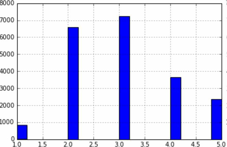
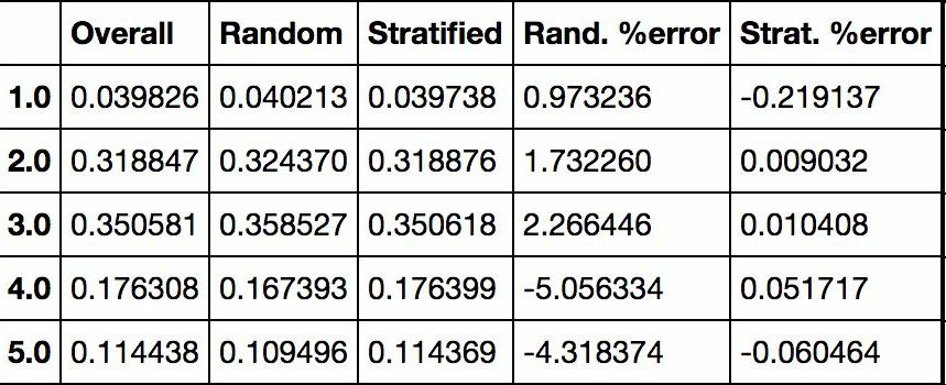
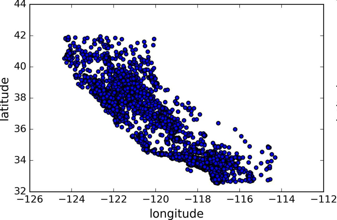
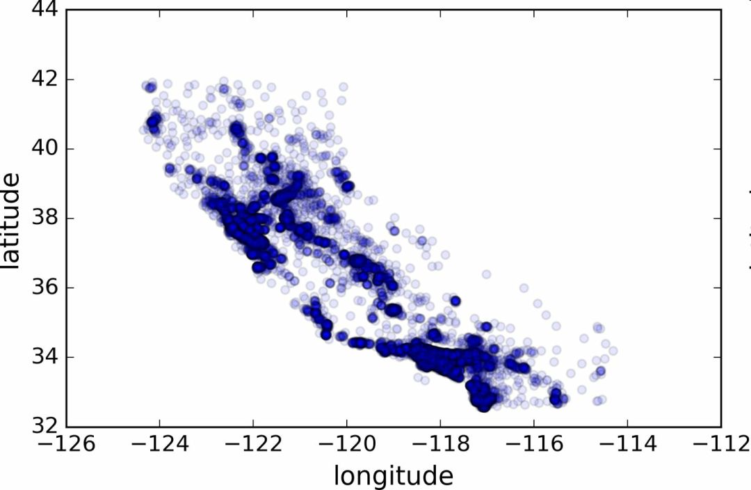
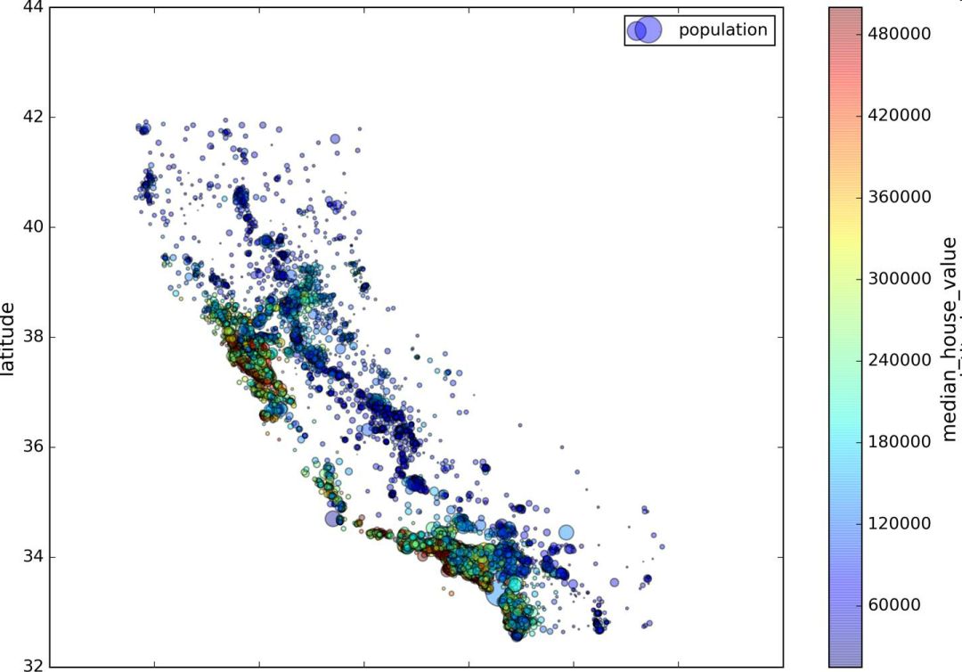
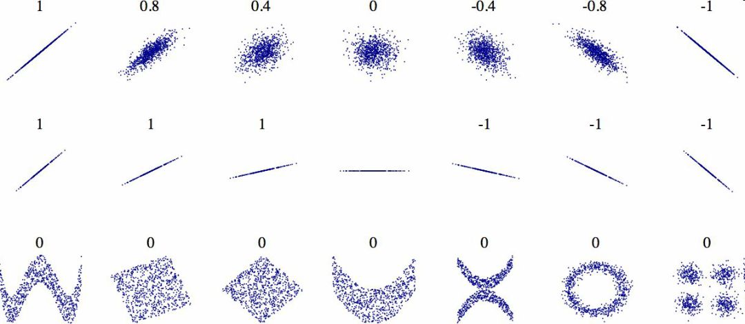
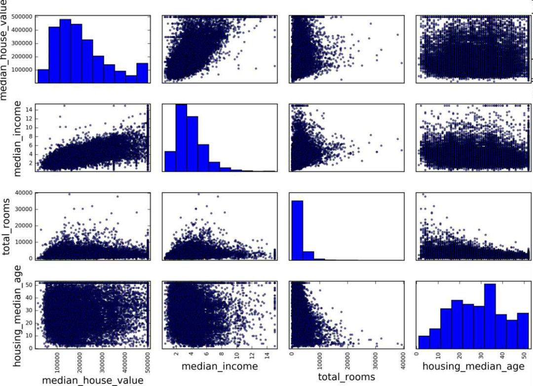
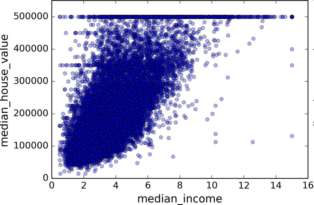
Create a test set Splitting the data at this stage sounds weird. After all, you just look at the data quickly and simply, and you need to investigate the data carefully to decide which algorithm to use. It is right to think so, but the human brain is a system of magical rules of discovery, which means that the brain is very prone to overfitting: if you look at the test set, you inadvertently choose one of the rules in the test set. Specific machine learning model. Again when you use the test set to assess the error rate, it will lead to an overly optimistic assessment, and the actual deployment of the system will be poor. This is called pivot deviation. In theory, creating a test set is straightforward: just randomly picking some instances, typically 20% of the data set, goes aside: Import numpy as np def split_train_test(data, test_ratio): shuffled_indices = np.random.permutation(len(data)) test_set_size = int(len(data) * test_ratio) test_indices = shuffled_indices[:test_set_size] train_indices = shuffled_indices[test_set_size:] Return data.iloc[train_indices], data.iloc[test_indices] Then you can use this function like this: >>> train_set, test_set = split_train_test(housing, 0.2) >>> print(len(train_set), "train +", len(test_set), "test") 16512 train + 4128 test This method works, but it is not perfect: if you run the program again, it will produce a different test set! After running multiple times, you (or your machine learning algorithm) will get the entire data set, which needs to be avoided. One of the solutions is to save the test set from the first run and load it in the subsequent process. Another approach is to set the seed of the random number generator (such as np.random.seed(42)) before calling np.random.permutation() to produce always the same shuffled indices. However, if the dataset is updated, both methods will fail. A common solution is to use the ID of each instance to determine if the instance should fit into the test set (assuming each instance has a unique and unchanging ID). For example, you can calculate the hash value of each instance ID, leaving only its last byte. If the value is less than or equal to 51 (20% of 256), it is put into the test set. This ensures that the test set remains unchanged in multiple runs, even if the data set is updated. The new test set will contain 20% of the new instances, but there will be no instances that were previously in the training set. Here is one of the available methods: Import hashlib def test_set_check(identifier, test_ratio, hash): return hash(np.int64(identifier)).digest()[-1] < 256 * test_ratio def split_train_test_by_id(data, test_ratio, id_column, hash=hashlib.md5): Ids = data[id_column] in_test_set = ids.apply(lambda id_: test_set_check(id_, test_ratio, hash)) return data.loc[~in_test_set], data.loc[in_test_set] However, the property dataset does not have an ID column. The easiest way is to use the row index as ID: Housing_with_id = housing.reset_index() # adds an `index` column train_set, test_set = split_train_test_by_id(housing_with_id, 0.2, "index") If you use a row index as the unique identifier, you need to ensure that the new data is placed at the end of the existing data, and no rows are deleted. If this is not possible, unique identifiers can be created with the most stable features. For example, the dimensions and longitude of a zone are constant for millions of years, so you can combine the two into one ID: Housing_with_id["id"] = housing["longitude"] * 1000 + housing["latitude"] train_set, test_set = split_train_test_by_id(housing_with_id, 0.2, "id") Scikit-Learn provides several functions that can be used to split a data set into multiple subsets. The simplest function is train_test_split. Its function is similar to the previous function split_train_test, with some other functions. First, it has a random_state parameter that can set the random generator seed mentioned earlier. Second, you can pass the seed to multiple datasets with the same number of rows. You can split the dataset on the same index (this function Very useful, for example, your tag value is placed in another DataFrame: From sklearn.model_selection import train_test_split train_set, test_set = train_test_split(housing, test_size=0.2, random_state=42) So far, we have adopted purely random sampling methods. When your data set is large (especially compared to the number of attributes), this is usually feasible; but if the data set is not large, there is a risk of sampling bias. When a survey company wants to investigate 1,000 people, they are not randomly selected in the phone booth for 1,000 people. The survey company needs to ensure that these 1,000 individuals are representative of the population as a whole. For example, 51.3% of the U.S. population is female and 48.7% are male. So in the United States, rigorous investigations need to ensure that the sample is also in this proportion: 513 women and 487 men. This is called stratified sampling: the population is divided into uniform sub-groups, called stratifications, and an appropriate number of instances are taken from each stratum to ensure that the test set is representative of the total number of people. If the survey company uses purely random sampling, there is a 12% probability of causing sampling bias: fewer than 49% or more than 54% of women. No matter what happens, the survey results will be seriously biased. Assume that the experts tell you that the median income is a very important attribute for predicting the median price. You may want to ensure that the test set can represent multiple revenue classifications in the overall data set. Because the median income is a continuous numeric attribute, you first need to create a revenue category attribute. Take a closer look at the histogram of the median income (Figure 2-9). (Annotation: This figure is a map after the median income has been processed): Figure 2-9 Bar Chart of Revenue Classification Most of the median income values ​​are clustered in 2-5 (ten thousand US dollars), but some of the median income will exceed 6. It is important that each tier in the dataset has enough instances in your data. Otherwise, the assessment of the importance of stratification will be biased. This means that you can't have too many layers, and each layer should be large enough. The following code creates a revenue category attribute by dividing the median income by 1.5 (to limit the number of income categories), rounding the values ​​with ceil (to produce a discrete classification), and then grouping all categories greater than 5 Into category 5: Housing["income_cat"] = np.ceil(housing["median_income"] / 1.5) housing["income_cat"].where(housing["income_cat"] < 5, 5.0, inplace=True) Now, stratified sampling can be based on income classification. You can use Scikit-Learn's StratifiedShuffleSplit class: From sklearn.model_selection import StratifiedShuffleSplit split = StratifiedShuffleSplit(n_splits=1, test_size=0.2, random_state=42) for train_index, test_index in split.split(housing, housing["income_cat"]): strat_train_set = housing.loc[train_index] strat_test_set = housing.loc[test_index] Check if the results meet expectations. You can view the revenue classification ratio in the complete property data set: >>> housing["income_cat"].value_counts() / len(housing) 3.0 0.350581 2.0 0.318847 4.0 0.176308 5.0 0.114438 1.0 0.039826 Name: income_cat, dtype: float64 Using a similar code, you can also measure the proportion of revenue classification in the test set. Figure 2-10 compares the revenue classification ratio of the total data set, the hierarchical sampling test set, and the pure random sampling test set. It can be seen that the proportion of revenue classification of the hierarchical sampling test set is almost the same as that of the total data set, while the deviation of the random sampling data set is serious. Figure 2-10 Comparison of sample biases between stratified sampling and pure random sampling Now you need to remove the income_cat attribute to bring the data back to the initial state: For set in (strat_train_set, strat_test_set): set.drop(["income_cat"], axis=1, inplace=True) The reason we used a lot of time to generate the test set is that the test set is usually ignored, but it is actually a very important part of machine learning. Also, many ideas in the process of generating test sets are very helpful for the following cross-validation discussions. Then go to the next stage: data exploration. Data exploration and visualization, discovery rules So far, you have just quickly looked at the data and have a general understanding of the data to be processed. The goal now is to explore data more deeply. First of all, make sure you put the test set aside and just study the training set. In addition, if the training set is very large, you may need to sample another exploration set to ensure that the operation is convenient and fast. In our case, the data set is small, so it can work directly on the universal set. Create a copy to avoid damaging the training set: Housing = strat_train_set.copy() Geographic data visualization Housing.plot(kind="scatter", x="longitude", y="latitude") Because of the geographic information (latitude and longitude), it is a good idea to create a scatter plot of all neighborhoods (Figure 2-11): Figure 2-11 Geographic Information Scatter Plot of Data This picture looks a lot like California, but I don't see any particular rules. Setting alpha to 0.1 makes it easier to see the density of data points (Figure 2-12): Figure 2-12 Scatter plot showing high density area It looks much better now: High-density areas can be seen very clearly, Bay Area, Los Angeles and San Diego, and Central Valley, especially from Sacramento and Fresno. Generally speaking, the human brain is very good at discovering the rules in the picture, but it needs to adjust the visualization parameters to make the rule appear. Now let's look at prices (Figure 2-13). The radius of each circle represents the population of the block (option s) and the color represents the price (option c). We use a predefined color chart named jet (option cmap). Its range is from blue (low price) to red (high price): Housing.plot(kind="scatter", x="longitude", y="latitude", alpha=0.4, s=housing["population"]/100, label="population", c="median_house_value", cmap =plt.get_cmap("jet"), colorbar=True, ) plt.legend() Figure 2-13 California House Prices This picture shows that house prices and locations (for example, by the sea) are closely related to population density, which you may already know. A clustering algorithm can be used to detect the main aggregation and a new feature value to measure the distance of the aggregation center. Although house prices in the northern California coastal area are not very high, the distance to sea property may also be useful, so this is not a problem that can be defined with a simple rule. Finding associations Because the data set is not very large, you can easily use the corr() method to calculate the standard correlation coefficient (also known as the Pearson correlation coefficient) between each pair of attributes: Corr_matrix = housing.corr() Now let's look at the correlation between each attribute and the median price: >>> corr_matrix["median_house_value"].sort_values(ascending=False) median_house_value 1.000000 median_income 0.687170 total_rooms 0.135231 housing_median_age 0.114220 households 0.064702 total_bedrooms 0.047865 population -0.026699 longitude -0.047279 latitude -0.142826 Name: median_house_value, dtype: float64 The range of the correlation coefficient is -1 to 1. When it approaches 1, it means strong positive correlation; for example, when the median income increases, the median price will increase. When the correlation coefficient is close to -1, it means strong negative correlation; as you can see, there is a slight negative correlation between latitude and median house price (that is, the further north, the lower the housing price may be). Finally, the correlation coefficient is close to 0, meaning there is no linear correlation. Figure 2-14 shows the different graphs of the correlation coefficient between the horizontal and vertical axes. Figure 2-14 Standard Correlation Coefficients for Different Datasets (Source: Wikipedia; Public Domain Pictures) Warning: The correlation coefficient only measures the linear relationship (if x rises, y rises or falls). The correlation coefficient may completely ignore the non-linear relationship (for example, if x is close to 0, the y value will become higher). In the last line of the above picture, their correlation coefficients are all close to 0, although their axes are not independent: these are examples of nonlinear relationships. In addition, the correlation coefficient of the second row is equal to 1 or -1; this has nothing to do with the slope. For example, the correlation coefficient between your height (in inches) and your height (in feet or nanometers) is 1. Another way to detect correlation coefficients between attributes is to use Pandas' scatter_matrix function, which draws a graph of each numeric attribute for each other numeric attribute. Because there are now 11 numerical attributes, you can get 11 ** 2 = 121 pictures that cannot be drawn on one page, so focus only on a few attributes that are most likely to be related to the median price of a house (Figure 2-15): From pandas.tools.plotting import scatter_matrix attributes = ["median_house_value", "median_income", "total_rooms", "housing_median_age"] scatter_matrix(housing[attributes], figsize=(12, 8)) Figure 2-15 Scatter matrix If pandas maps each variable to itself, the main diagonal (upper left to lower right) will be a straight line. So Pandas shows a histogram of each property (otherwise, please refer to the Pandas documentation). The most promising property used to predict the median price is the median income, so this map is enlarged (Figure 2-16): Housing.plot(kind="scatter", x="median_income",y="median_house_value", alpha=0.1) Figure 2-16 Median income vs median house price This picture illustrates a few points. First of all, the correlation is very high; the upward trend can be clearly seen, and the data points are not very scattered. Second, the highest price we saw before was clearly presented as a horizontal line at $500000. This figure also shows some less obvious straight lines: a straight line at $450000, a straight line at $350000, a line at $280000, and some more downline. You may wish to remove the corresponding block to prevent the algorithm from repeating these coincidences. Attribute combination test It is hoped that the previous energy conservation will teach you some ways to explore the data and discover the laws. You have discovered the coincidence of some data and need to remove it before providing it to the algorithm. You also discovered interesting associations between attributes, especially the target attributes. You also notice that some attributes have a long tail distribution, so you may want to convert them (for example, calculate their log logarithms). Of course, the treatment of different projects is different, but the general idea is similar. The last thing you need to do before preparing the data for the algorithm is to try out a combination of properties. For example, if you don't know how many houses are in a given block, the total number of rooms in that block is useless. What you really need is a few rooms per household. Similarly, the total number of bedrooms is not important: you may need to compare it with the number of rooms. The number of people in each household is also an interesting combination of attributes. Let's create these new properties: Housing["rooms_per_household"] = housing["total_rooms"]/housing["households"] housing["bedrooms_per_room"] = housing["total_bedrooms"]/housing["total_rooms"] housing["population_per_household"]=housing[" Population"]/housing["households"] Now let's look at the correlation matrix: >>> corr_matrix = housing.corr() >>> corr_matrix["median_house_value"].sort_values(ascending=False) median_house_value 1.000000 median_income 0.687170 rooms_per_household 0.199343 total_rooms 0.135231 housing_median_age 0.114220 households 0.064702 total_bedrooms 0.047865 population_per_household -0.021984 population -0.026699 longitude -0.047279 latitude -0.142826 bedrooms_per_room -0.260070 Name: median_house_value, dtype: float64 Looks good! The new bedrooms_per_room attribute is more strongly associated with the median house price than the total number of rooms or the number of bedrooms. Obviously, the lower the number of bedrooms/total rooms, the higher the price. The number of rooms in each household is also more informative than the total number of rooms in the neighborhood. Obviously, the larger the house, the higher the price. The data exploration in this step does not have to be very complete. The purpose here is to have a correct start, to quickly discover the laws and to get a reasonable prototype. But this is an interactive process: once you get a prototype and run it, you can analyze its output, find more rules, and then return to data exploration. Octagonal Steel Pole,Octagonal Steel Pole For Medium-Voltage Lines,Galvanized Longitudinal Welded Steel Pole,Octagonal Galvanized Steel Pole Jiangsu Baojuhe Science and Technology Co.,Ltd. , https://www.galvanizedsteelpole.com